 

Find the shortcut. Learn the biology.
Automated quality control for genomic machine learning datasets: scores the biases, duplicates and data leakage a classifier could exploit before you train on it.
When the classes differ in something trivial, a high score no longer tells you
what a model learned — the biology, or the shortcut. gb-qc looks for the
differences a classifier could exploit without understanding anything: classes
that differ in length or base composition, a give-away at a single position, the
same sequence in both classes, a test set that repeats the training set.
pip install genomic-benchmarks-qc
Python 3.12 or newer; the leakage check wants one extra thing — see installation.
Point it at your own dataset, or fetch the two enhancers files to run the command below exactly as it stands:
curl -fLO https://raw.githubusercontent.com/genomic-benchmarks/genomic-benchmarks-qc/main/examples/enhancers/data/enhancers_train.csv
curl -fLO https://raw.githubusercontent.com/genomic-benchmarks/genomic-benchmarks-qc/main/examples/enhancers/data/enhancers_test.csv
gb-qc evaluate-classes \
  --input enhancers_train.csv \
  --input enhancers_test.csv \
  --out-folder qc-out
Every check gets a Pass, Warning or Fail flag, a standalone HTML report you can read or mail, and a CSV you can put in CI.
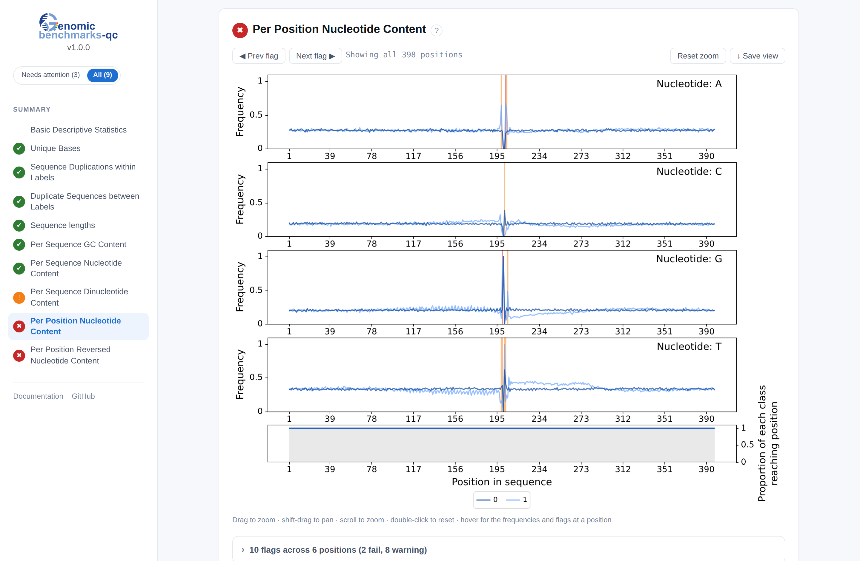
The report for hidden-motif, one of the eight worked examples below — click it to open the real one. Six of its nine checks pass: length, GC content and base composition are all clean, and the entire finding is that spike halfway along. The panel is interactive because it has to be — at this width the flagged region is a hairline. Everything is in the one file: no server, no assets directory, nothing to host.
Start here
-
A flag fired. Now what?
The checks — what each one measures, and what to actually do about it. The page to read first.
-
Why should I trust a flag?
How a flag is decided — the single-feature AU-ROC, the 0.6 and 0.7 boundaries, and why Unknown is not Pass.
-
Show me it working
Eight worked examples with live reports. Start with hidden-motif, whose only flaw is six positions wide.
-
Something is wrong
Troubleshooting — MMseqs2 not found, everything came back
Unknown, it is slow, the plot stops early.
The examples
Eight datasets, each the only one that shows a particular thing, with flags measured rather than asserted. They are the fastest way to see what a report actually tells you — start with the overview, or go straight to a report below.
| Example | What it shows | Report |
|---|---|---|
clean-dataset |
The control: what "nothing wrong" looks like, AU-ROC 0.50–0.54 throughout | open |
composition-bias |
The worst case — six checks fail, and 6% of the test set is already in training | open |
hidden-motif |
A bias six positions wide inside 398 positions. Why the per-position plot is interactive | open |
variable-length |
Sequences that stop at different places, and why most positions go unscored | open |
length-bias |
Length alone separating the classes, on a continuous label | open |
paired-sequences |
Two sequence columns in one row | open |
fasta-classes |
One FASTA file per class | open |
enhancers |
The quickstart dataset, with a little real train/test leakage | open |
Each has a page of its own explaining what the dataset is,
the exact command, and what a reader should conclude. The data and its
provenance live in
examples/;
the reports are built from it by the same commands shown there, so what you read
is always what the current code produces.
Flags
Flags come from the AU-ROC of a classifier that sees only the one feature under test — see how a flag is decided for why the boundaries sit where they do:
| Flag | AU-ROC | Meaning |
|---|---|---|
| Pass | ≤ 0.6 | Classes not distinguishable by this feature |
| Warning | ≤ 0.7 | A model could get some traction here |
| Fail | > 0.7 | Significant bias detected |
| Unknown | — | Not enough sequences to score the check |
Unknown is not Pass. It says the comparison was not made, not that it came out clean — a check needs at least 250 sequences per class before it is scored at all. The plots and descriptive statistics are computed from all the data either way, so a small dataset can still be compared by eye.
Also here
- The per-position plot — it is interactive, and one example explains why it has to be
- Train/test leakage — how similarity is measured, and what to do about it
- Using it in CI — the CSV as a build gate
- Python API — both commands are one function call